C++ BFS/DFS Code Implementation Tutorial

4/3/2018

Introduction: Graph Algorithms

A lot of problems in real life are modeled as graphs, and we need to be able to represent those graphs in our code. In this (short) tutorial, we're going to go over graphs, representing those graphs as adjacency lists/matrices, and then we'll look at using Breadth First Search (BFS) and Depth First Search (DFS) to traverse a graph. We'll be writing our code in C++, although the concepts can be extended to any programming language.

This tutorial is supposed to focus on the code, so the drawings are going to be ugly, and the definitions are going to be quick reminders instead of in-depth explanations.

Graphs

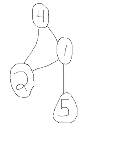
To put it simply, graphs are a set of edges that connect some vertices. To say it "less mathy", there are some points, and some lines that connect those points.

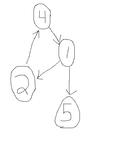
In the graph above, we have four vertices (4, 1, 2, 5) that are connected by some edges. In this case, the edges are bidirectional, meaning 1 is connected to 4 and 4 is connected to 1. Some graphs have directed edges, meaning travel is only allowed in one direction.

Now someone at node 4 can get to node 1, but node 1 can't directly travel to node 4.

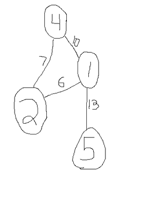
Finally, sometimes edges have weights on them.

A reason edges would have weights are to represent distances, as an example. For instance, one road could be 10 miles long, and another is 13.

So how do we represent these graphs in our code? We create what are called adjacency matrices and adjacency lists.

Adjacency Matrices

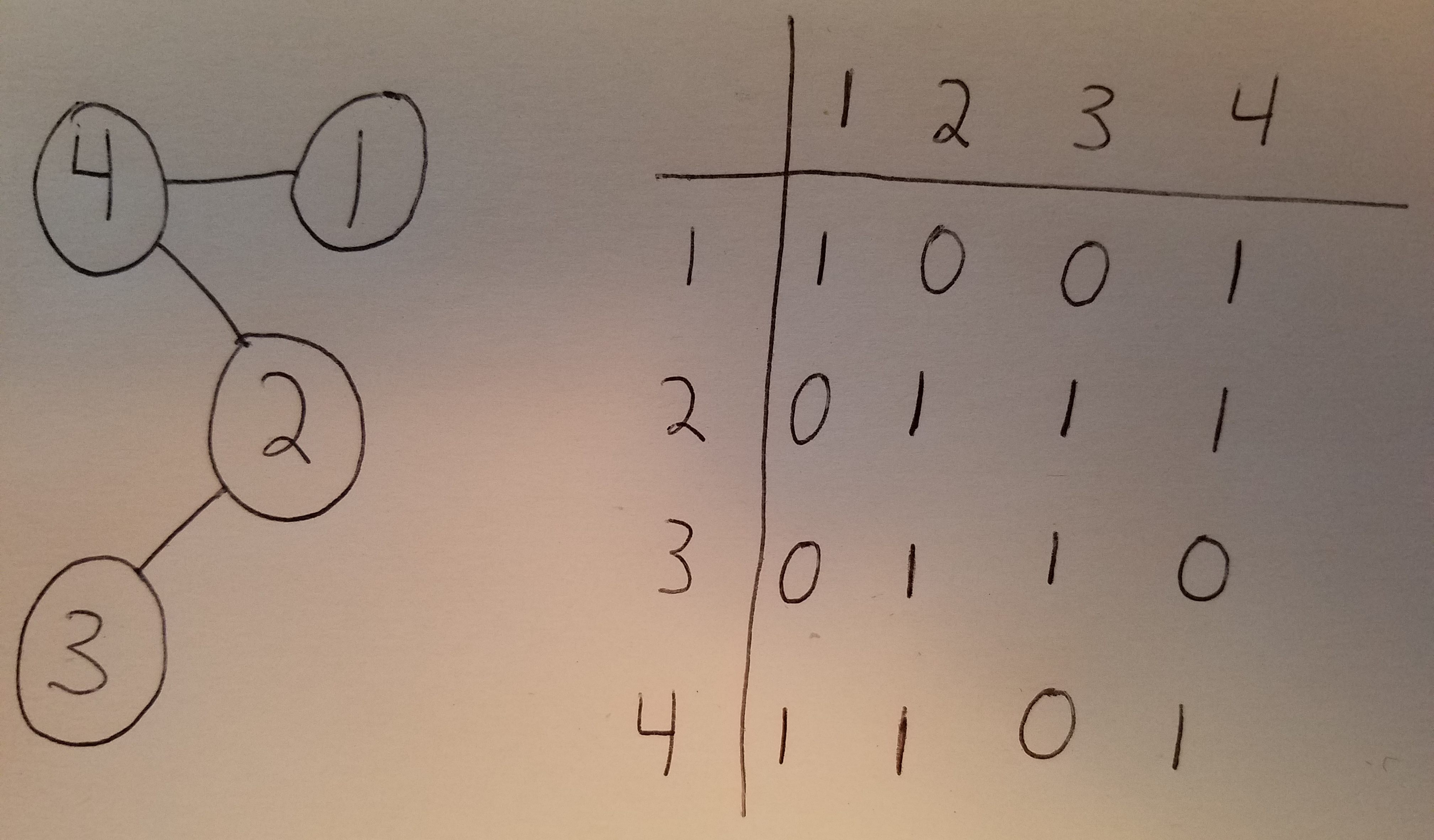
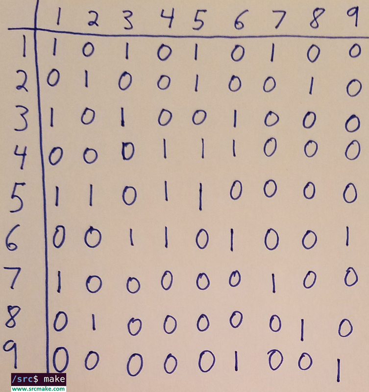
An adjacency matrix is basically a table/spreadsheet, where each row and column represent a vertex. If the vertex 1 and vertex 4 are connected, then cell (1, 4) is a 1. If they aren't connected, then the cell is a 0.

If there's a certain edge weight, then you can represent that edge weight instead of 1 in the cell.

Adjacency matrices take up O(N^2) space. To find if a connection between two vertices exist takes O(1) time, since it's a quick lookup in the table. To add a vertex takes O(N) time, since you need to add a whole row for the new vertex (which also means initialization of the graph takes O(N^2) time).

Adjacency Lists

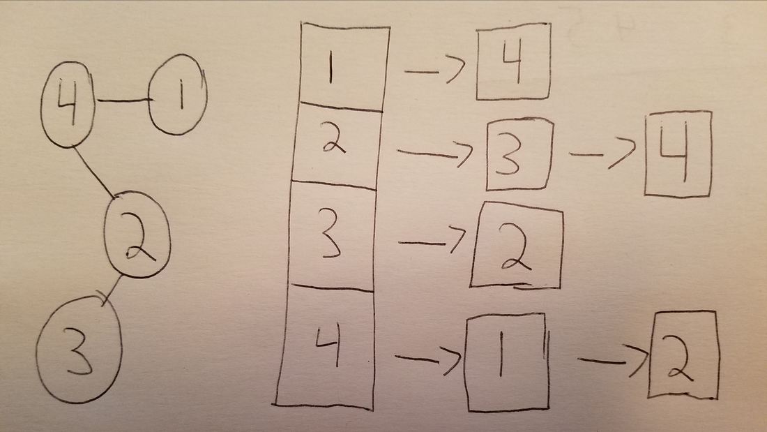
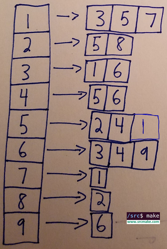
An adjacency list is another way to represent the edges of a graph. You create a list/array/vector that represents each vertex, and inside of each index for that vertex exists another list/vector/array for all of the vertices that the owner is connected too.

An adjacency list takes up less space than an adjacency matrix. The actual space it takes up varies based on the graph, but in the worse case, it could take up O(N^2) space if all vertices are connected to each other, which makes it MUCH worse than an adjacency matrix.

To look up a connection takes up O(N) time, as you have to search through a vertex's friend list to see if the friend exists. To add a new vertex is simple, though, and takes O(1) time, since you're just adding it to the end of a list.

Traversing The Graph

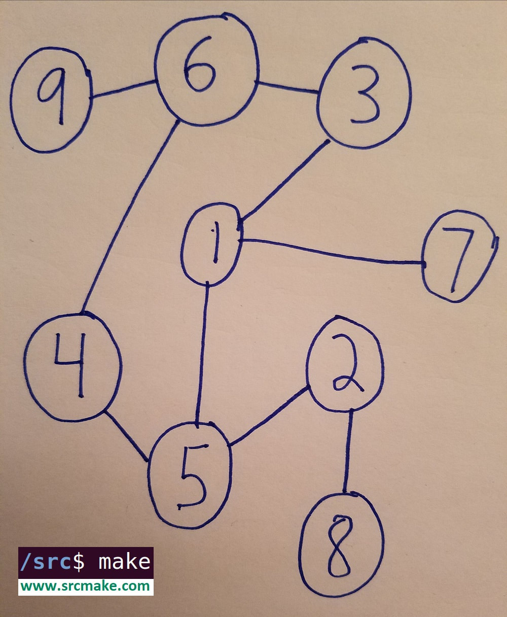
So we can represent graphs in our code. (Well, you'll see the coding representations soon.) But how do we traverse through a graph? Specifically, if we're at vertex 1, can we get to vertex 3? What path do we take?

To traverse through a graph, we use BFS and DFS. For the sake of our examples, we're going to traverse through the following graph:

A graph. (Undirected. Unweighted.)

Adjacency Matrix form of the graph.

Adjacency List form of the graph.

Breadth First Search (BFS)

BFS is a technique for traversing through a graph where we start at a certain vertex, visit all of that vertex's neighbors, then visit the neighbor's neighbors, then visit the neighbor's neighbor's neighbors, etc. (In that order.)

// Copyright srcmake 2018.
// C++ Example Breadth First Search (BFS) Code. And Adjacency Lists.
/* BFS concept: In a graph, starting from a certain node, visit all other nodes.
The order of visiting is "all of my friends first, then my friends friends".
*/

/* BFS coding:
// Create a "visited" array (true or false) to keep track of if we visited a vertex.
// Create a queue for the nodes we visit.
// Add the starting vertex to the queue and mark it as visited.
// While the queue is not empty..
    // Loop through all of it's friends.
        // If the friend hasn't been visited yet, add it to the queue and mark it as visited.
*/

// The example graph: https://www.srcmake.com/uploads/5/3/9/0/5390645/graph_orig.jpg

#include <iostream>
#include <vector>
#include <queue>

using namespace std;

// Adjacency List - Adding O(1), Lookup O(N), Space O(N^2) but usually better.
// Each vector position represents a node - the vector inside that position represents that node's friends.
vector< vector<int> > FormAdjList()
    {
    // Our adjacency list.
    vector< vector<int> > adjList;
    
    // We have 10 vertices, so initialize 10 rows.
    const int n = 9;
    
    for(int i = 0; i < n; i++)
        {
        // Create a vector to represent a row, and add it to the adjList.
        vector<int> row;
        adjList.push_back(row);
        }
    
    // Now "adjList[0]" has a vector<int> in it that represents the friends of vertex 1. 
    // (Remember, we use 0-based indexing. 0 is the first number in our vector, not 1.
    
    // Now let's add our actual edges into the adjacency list.
    // See the picture here: https://www.srcmake.com/uploads/5/3/9/0/5390645/adjl_4_orig.png
    
    adjList[0].push_back(2);
    adjList[0].push_back(4);
    adjList[0].push_back(6);
    
    adjList[1].push_back(4);
    adjList[1].push_back(7);
    
    adjList[2].push_back(0);
    adjList[2].push_back(5);
    
    adjList[3].push_back(4);
    adjList[3].push_back(5);
    
    adjList[4].push_back(1);
    adjList[4].push_back(3);
    adjList[4].push_back(0);
    
    adjList[5].push_back(2);
    adjList[5].push_back(3);
    adjList[5].push_back(8);
    
    adjList[6].push_back(0);
    
    adjList[7].push_back(1);
    
    adjList[8].push_back(5);
    
    // Our graph is now represented as an adjacency list. 
    return adjList;
    }
    
// Adjacency Matrix - Adding O(N), Lookup O(1), Space O(N^2)
vector< vector<int> > FormAdjMatrix()
    {
    // We could use an array for the adjMatrix if we knew the size, but it's safer to use a vector.
    vector< vector<int> > adjMatrix;
    
    // Initialize the adjMatrix so that all vertices can visit themselves.
    // (Basically, make an identity matrix.)
    const int n = 9;
    
    for(int i = 0; i < n; i++)
        {
        // Initialize the row.
        vector<int> row;
        adjMatrix.push_back(row);
        
        // Set the row to have all 0's. (Except the vertex ing itself.)
        for(int j = 0; j < n; j++)
            {
            int value = 0;
            
            if(i == j) 
                { value = 1; }
            
            adjMatrix[i].push_back(value);
            }
        }
    
    // Our matrix is set up, we just need to set up the edges (vertex connections).
    // See this image: https://www.srcmake.com/uploads/5/3/9/0/5390645/adjm_2_orig.png
    
    adjMatrix[0][2] = 1;
    adjMatrix[2][0] = 1;
    
    adjMatrix[0][4] = 1;
    adjMatrix[4][0] = 1;
    
    adjMatrix[0][6] = 1;
    adjMatrix[6][0] = 1;
    
    adjMatrix[1][4] = 1;
    adjMatrix[4][1] = 1;
    
    adjMatrix[1][7] = 1;
    adjMatrix[7][1] = 1;
    
    adjMatrix[2][5] = 1;
    adjMatrix[5][2] = 1;
    
    adjMatrix[3][4] = 1;
    adjMatrix[4][3] = 1;
    
    adjMatrix[3][5] = 1;
    adjMatrix[5][3] = 1;
    
    adjMatrix[5][8] = 1;
    adjMatrix[8][5] = 1;
    
    // Our adjacency matrix is complete.
    return adjMatrix;
    }
    
// Given an Adjacency List, do a BFS on vertex "start"
void AdjListBFS(vector< vector<int> > adjList, int start)
    {
    cout << "\nDoing a BFS on an adjacency list.\n";
    
    int n = adjList.size();
    // Create a "visited" array (true or false) to keep track of if we visited a vertex.
    bool visited[n] = { false };
    
    // Create a queue for the nodes we visit.
    queue<int> q;
    
    // Add the starting vertex to the queue and mark it as visited.
    q.push(start);
    visited[start] = true;
    
    // While the queue is not empty..
    while(q.empty() == false)
        {
        int vertex = q.front();
        q.pop();
        
        // Doing +1 in the cout because our graph is 1-based indexing, but our code is 0-based.
        cout << vertex+1 << " ";
        
        // Loop through all of it's friends.
        for(int i = 0; i < adjList[vertex].size(); i++)
            {
            // If the friend hasn't been visited yet, add it to the queue and mark it as visited
            int neighbor = adjList[vertex][i];
            
            if(visited[neighbor] == false)
                {
                q.push(neighbor);
                visited[neighbor] = true;
                }
            }
        }
    cout << endl << endl;
    return;
    }
    
    
// Given an Adjacency Matrix, do a BFS on vertex "start"
void AdjMatrixBFS(vector< vector<int> > adjMatrix, int start)
    {
    cout << "\nDoing a BFS on an adjacency list.\n";
    
    int n = adjMatrix.size();
    // Create a "visited" array (true or false) to keep track of if we visited a vertex.
    bool visited[n] = { false };
    
    // Create a queue for the nodes we visit.
    queue<int> q;
    
    // Add the starting vertex to the queue and mark it as visited.
    q.push(start);
    visited[start] = true;
    
    // While the queue is not empty..
    while(q.empty() == false)
        {
        int vertex = q.front();
        q.pop();
        
        // Doing +1 in the cout because our graph is 1-based indexing, but our code is 0-based.
        cout << vertex+1 << " ";
        
        // Loop through all of it's friends.
        for(int i = 0; i < adjMatrix[vertex].size(); i++)
            {
            
            // The neighbor is the column number, and the edge is the value in the matrix.
            int neighbor = i;
            int edge = adjMatrix[vertex][i];
            
            // If the edge is "0" it means this guy isn't a neighbor. Move on.
            if(edge == 0) { continue; }
            
            // If the friend hasn't been visited yet, add it to the queue and mark it as visited
            if(visited[neighbor] == false)
                {
                q.push(neighbor);
                visited[neighbor] = true;
                }
            }
        }
    cout << endl << endl;
    return;
    }
    
int main() 
    {
    cout << "Program started.\n";
    
    // Get the adjacency list/matrix.
    vector< vector<int> > adjList = FormAdjList();
    vector< vector<int> > adjMatrix = FormAdjMatrix();
    
    // Call BFS on Vertex 5. (Labeled as 4 in our 0-based-indexing.)
    AdjListBFS(adjList, 4);
    AdjMatrixBFS(adjMatrix, 4);
    
    cout << "Program ended.\n";
    
    return 0;
    }

Read through the comments to see what's going on.

Depth First Search (DFS)

Similar to BFS, DFS is a way to traverse a graph. However, instead of using a visiting all of a vertices neighbors before visiting the neighbor's neighbors, DFS just keeps visiting each new node it sees, meaning that it will usually go down a long path, and then come back to visit what it missed. As opposed to a queue, DFS works using recursion.

// Copyright srcmake 2018.
// C++ Example Depth First Search (DFS) Code. And Adjacency Lists/Matrixes.
/* DFS concept: In a graph, starting from a certain node, visit all other nodes.
The order of visiting is "all of my friends first, then my friends friends".
*/

/* DFS coding:
// Create a "visited" array (true or false) to keep track of if we visited a vertex.

Recursively call DFS(vertex, visited, adjList/Matrix), which for each node...
    // Marks it as visited
    // Checks for all neighbors...
    // Makes a recursive call if the neighbor is not visited.
*/

// The example graph: https://www.srcmake.com/uploads/5/3/9/0/5390645/graph_orig.jpg

#include <iostream>
#include <vector>

using namespace std;

//////////////////////////////////////////////////////////////////////////////////////////////
// Adjacency List - Adding O(1), Lookup O(N), Space O(N^2) but usually better.
// Each vector position represents a node - the vector inside that position represents that node's friends.
vector< vector<int> > FormAdjList()
    {
    // Our adjacency list.
    vector< vector<int> > adjList;
    
    // We have 10 vertices, so initialize 10 rows.
    const int n = 9;
    
    for(int i = 0; i < n; i++)
        {
        // Create a vector to represent a row, and add it to the adjList.
        vector<int> row;
        adjList.push_back(row);
        }
    
    // Now "adjList[0]" has a vector<int> in it that represents the friends of vertex 1. 
    // (Remember, we use 0-based indexing. 0 is the first number in our vector, not 1.
    
    // Now let's add our actual edges into the adjacency list.
    // See the picture here: https://www.srcmake.com/uploads/5/3/9/0/5390645/adjl_4_orig.png
    
    adjList[0].push_back(2);
    adjList[0].push_back(4);
    adjList[0].push_back(6);
    
    adjList[1].push_back(4);
    adjList[1].push_back(7);
    
    adjList[2].push_back(0);
    adjList[2].push_back(5);
    
    adjList[3].push_back(4);
    adjList[3].push_back(5);
    
    adjList[4].push_back(1);
    adjList[4].push_back(3);
    adjList[4].push_back(0);
    
    adjList[5].push_back(2);
    adjList[5].push_back(3);
    adjList[5].push_back(8);
    
    adjList[6].push_back(0);
    
    adjList[7].push_back(1);
    
    adjList[8].push_back(5);
    
    // Our graph is now represented as an adjacency list. 
    return adjList;
    }
//////////////////////////////////////////////////////////////////////////////////////////////
    
    
//////////////////////////////////////////////////////////////////////////////////////////////
// Adjacency Matrix - Adding O(N), Lookup O(1), Space O(N^2)
vector< vector<int> > FormAdjMatrix()
    {
    // We could use an array for the adjMatrix if we knew the size, but it's safer to use a vector.
    vector< vector<int> > adjMatrix;
    
    // Initialize the adjMatrix so that all vertices can visit themselves.
    // (Basically, make an identity matrix.)
    const int n = 9;
    
    for(int i = 0; i < n; i++)
        {
        // Initialize the row.
        vector<int> row;
        adjMatrix.push_back(row);
        
        // Set the row to have all 0's. (Except the vertex ing itself.)
        for(int j = 0; j < n; j++)
            {
            int value = 0;
            
            if(i == j) 
                { value = 1; }
            
            adjMatrix[i].push_back(value);
            }
        }
    
    // Our matrix is set up, we just need to set up the edges (vertex connections).
    // See this image: https://www.srcmake.com/uploads/5/3/9/0/5390645/adjm_2_orig.png
    
    adjMatrix[0][2] = 1;
    adjMatrix[2][0] = 1;
    
    adjMatrix[0][4] = 1;
    adjMatrix[4][0] = 1;
    
    adjMatrix[0][6] = 1;
    adjMatrix[6][0] = 1;
    
    adjMatrix[1][4] = 1;
    adjMatrix[4][1] = 1;
    
    adjMatrix[1][7] = 1;
    adjMatrix[7][1] = 1;
    
    adjMatrix[2][5] = 1;
    adjMatrix[5][2] = 1;
    
    adjMatrix[3][4] = 1;
    adjMatrix[4][3] = 1;
    
    adjMatrix[3][5] = 1;
    adjMatrix[5][3] = 1;
    
    adjMatrix[5][8] = 1;
    adjMatrix[8][5] = 1;
    
    // Our adjacency matrix is complete.
    return adjMatrix;
    }
//////////////////////////////////////////////////////////////////////////////////////////////
    
    
//////////////////////////////////////////////////////////////////////////////////////////////    
// Recursively visit vertices. 
void AdjListDFS(vector< vector<int> > &adjList, int &vertex, vector<bool> &visited)
    {
    // Mark the vertex as visited.
    visited[vertex] = true;
    
    // Outputting vertex+1 because that's the way our graph picture looks.
    cout << vertex+1 << " ";
    
    // Look at this vertex's neighbors.
    for(int i = 0; i < adjList[vertex].size(); i++)
        {
        int neighbor = adjList[vertex][i];
        // Recursively call DFS on the neighbor, if it wasn't visited.
        if(visited[neighbor] == false)
            {
            AdjListDFS(adjList, neighbor, visited);
            }
        }
    }
    
// Given an Adjacency List, do a BFS on vertex "start"
void AdjListDFSInitialize(vector< vector<int> > &adjList, int start)
    {
    cout << "\nDoing a DFS on an adjacency list.\n";
    
    int n = adjList.size();
    // Create a "visited" array (true or false) to keep track of if we visited a vertex.
    vector<bool> visited;
    
    for(int i = 0; i < n; i++)
        {
        visited.push_back(false);
        }
    
    AdjListDFS(adjList, start, visited);
    
    cout << endl << endl;
    return;
    }
//////////////////////////////////////////////////////////////////////////////////////////////


//////////////////////////////////////////////////////////////////////////////////////////////
// Recursively visit vertices. 
void AdjMatrixDFS(vector< vector<int> > &adjMatrix, int &vertex, vector<bool> &visited)
    {
    // Mark the vertex as visited.
    visited[vertex] = true;
    
    // Outputting vertex+1 because that's the way our graph picture looks.
    cout << vertex+1 << " ";
    
    // Look at this vertex's neighbors.
    for(int i = 0; i < adjMatrix[vertex].size(); i++)
        {
        int edge = adjMatrix[vertex][i];
        int neighbor = i;
        //cout << "Neighbor: " << i << endl;
        // If the edge doesn't exist, move on.
        if(edge == 0) { continue; }
        
        // Recursively call DFS on the neighbor, if it wasn't visited.
        if(visited[neighbor] == false)
            {
            AdjMatrixDFS(adjMatrix, neighbor, visited);
            }
        }
    }
    
// Given an Adjacency Matrix, do a BFS on vertex "start"
void AdjMatrixDFSInitialize(vector< vector<int> > &adjMatrix, int start)
    {
    cout << "\nDoing a DFS on an adjacency matrix.\n";
    
    int n = adjMatrix.size();
    // Create a "visited" array (true or false) to keep track of if we visited a vertex.
    vector<bool> visited;
    
    for(int i = 0; i < n; i++)
        {
        visited.push_back(false);
        }
    
    AdjMatrixDFS(adjMatrix, start, visited);
    
    cout << endl << endl;
    return;
    }
//////////////////////////////////////////////////////////////////////////////////////////////


//////////////////////////////////////////////////////////////////////////////////////////////    
int main() 
    {
    cout << "Program started.\n";
    
    // Get the adjacency list/matrix.
    vector< vector<int> > adjList = FormAdjList();
    vector< vector<int> > adjMatrix = FormAdjMatrix();
    
    // Call BFS on Vertex 5. (Labeled as 4 in our 0-based-indexing.)
    AdjListDFSInitialize(adjList, 4);
    AdjMatrixDFSInitialize(adjMatrix, 4);
    
    cout << "Program ended.\n";
    
    return 0;
    }
//////////////////////////////////////////////////////////////////////////////////////////////

Read the comments to see how it works.

Conclusion

We went over Graphs, Adjacency Lists, Adjacency Matrices, BFS, and DFS. These data structures and traversal techniques are vital to using graphs.

The next step is to learn about calculating the shortest paths in graphs. See the next blog post to do this.

Then, take a look at maximum flow in this blog post..

Like this content and want more? Feel free to look around and find another blog post that interests you. You can also contact me through one of the various social media channels.

Twitter: @srcmake
Discord: srcmake#3644
Youtube: srcmake
Twitch: www.twitch.tv/srcmake
Github: srcmake

Comments are closed.

Author

Hi, I'm srcmake. I play video games and develop software.

Pro-tip: Click the "DIRECTORY" button in the menu to find a list of blog posts.

License: All code and instructions are provided under the MIT License.

Discord

Chat with me.

Youtube

Watch my videos.

Twitter

Get the latest news.

Twitch

See the me code live.

Github

My latest projects.